Dataflow Code Generation for HLS
The following topics are covered in this tutorial:
- Implementation of a Gaussian difference filter using streaming actors
- Code generation for Xilinx FPGA using Preesm
Prerequisite:
- Preesm installation
- Vitis HLS 2021.2, required for timing estimation and hardware synthesis, tested on Ubuntu 20.04
- Previous Preesm tutorials will help understanding the notions of workflow, scenario, etc.
Tutorial created the 17.04.2023 by M. Dardaillon
Project Setup
- Download the Gaussian difference project on github.
- Launch Preesm and open the project using “File > open Projects from File Systems…”.
- Select the project and import it.
- To see the graph hereunder, generate the
gaussian_difference.diagramfile by right clicking thegaussian_difference.pifile and selectingPreesm/generate .diagram file; then double click thegaussian_difference.diagramfile.
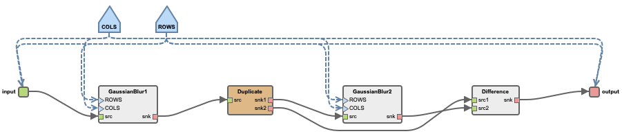
Please note that contrary to the previous Preesm graph examples, this top graph has input and output ports, as Preesm generates acceleration code to be fed data by an external process.
Application development
Preesm applications targeting FPGA are based on static dataflow, support hierarchy, parameters specified at synthesis time and cycles using delays. The main difference compared to applications targeting CPU is the use of HLS oriented C++ code inside actors to be synthesizable by Xilinx Vitis HLS. Of special note is the use of hls::stream<> instead of pointers on all inputs and outputs of an actor. Streams hls::stream<> are implemented as fifos in Xilinx, and can be accessed with read() and write() methods. A simple example can be seen in the Difference actor, by double clicking on it to access its implementation.
Another important difference with CPU-based application is the two timings used to characterize an actor:
- Execution Time: the number of cycles for an actor to execute completely, from reading its first input to writing its last output
- Initiation Interval: the number of cycles for an actor to start a new execution, with the actor potentially still processing previous executions using an internal pipeline.
These timings are set in the scenario file.
Given the use of streams fifos reading/writing a single token per cycle, those timings need to be at least equal or superior to the maximum number of tokens on all inputs/outputs of the given actor. Those timings currently need to be manually extracted from Vitis HLS using a synthesis to be reported on the scenario content.
Timings can be observed for the Gaussian difference application in the included scenario in the Timings tab. The annotated timings are for a PYNQ Z2 target clocked at 100 MHz. The Difference actor is implemented at the pixel granularity and takes only 1 cycle to execute, while the GaussianBlur actors are implemented at the image level and take 390072 cycles to execute. The analysis methods for dataflow HLS are not sensitive to large repetition counts and benefit from finer granularity such as the Difference actor to reach more efficient implementation.
Application synthesis
Application synthesis is performed in 2 steps, 1. by generating a C++ implementation for HLS using Preesm, 2. by performing an hardware synthesis using Vitis and Vitis HLS.
HLS implementation generation
From Preesm, the application can be synthesized using the FPGAAnalysis.workflow. The FPGA Analysis whorkflow task has 2 main parameters:
- Fifo evaluator is based on ADFG analysis and determines automatically the required FIFO sizes to guarantee the absence of deadlock and reach maximal throughput. It can be set to
adfgFifoEvalExactfor the most precise analysis, oradfgFifoEvalLinearfor an overestimation in case the ILP solver overflows on more complex graphs. - Pack tokens is a technique to minimize BRAM usage by FIFOs by packing multiple tokens together in a single FIFO stored value, trading BRAM usage for a small increase in latency.
Launch the synthesis by running the workflow on gaussian_difference.scenario. This should take a few seconds. During synthesis, each actor is implemented independently with no resource sharing between actors. They are connected using FIFOs as dimensioned by ADFG and displayed in the log with their sizes given in bits.
Hardware synthesis for PYNQ
Follow these steps to generate the final hardware implementation:
- Open a terminal with the Xilinx toolchain included in the PATH;
- Navigate to the Gaussian difference application folder;
- Navigate to
Code/generated/inside the application folder; - Run
make all, the synthesis should take a few minutes.
In the previous step, Preesm implemented all actors and connected them with FIFOs. Additionally, the graph is interfaced with the CPU on the Zynq platform using DMAs in mem_read_gaussian_difference.cpp and mem_write_gaussian_difference.cpp, with array interfaces for the CPU application. A platform is automatically generated to support this interface, with 3 different hosts:
- An OpenCL host
host_xocl_gaussian_difference.cppto support OpenCL hardware acceleration; - A bare metal C host
host_c_gaussian_difference.cppfor low level, low latency implementation; - A Python host
host_pynq_gaussian_difference.ipynbbased on Xilinx PYNQ for ease of use.
Deployment on PYNQ
Follow these steps to deply on PYNQ:
- Copy the following 3 files in the same folder on the PYNQ board:
- The Jupyter notebook to run
host_pynq_gaussian_difference.ipynb - The FPGA bitfile
gaussian_difference.bit - The FPGA bitfile interface for PYNQ
gaussian_difference.hwh
- The Jupyter notebook to run
- Open
host_pynq_gaussian_difference.ipynbin the editor; - Replace
TODO fill datato read animage.jpgof size 720 x 540 in Python, convert it to B&W and load the pixel values ininput_vectto be transfered on the FPGA;
from PIL import Image
input_buff = allocate(shape=(RATE_OF_INPUT,), dtype=np.dtype(np.uint8))
img = Image.open('image.jpg)'
img = img.convert('L')
input_vect = np.array(img)
input_vect = input_vect.reshape(RATE_OF_INPUT)
np.copyto(input_buff, input_vect)

output_buff = allocate(shape=(RATE_OF_OUTPUT,), dtype=np.dtype(np.uint8))
- Replace
TODO check resultsto display a B&W image in Python based on the values in output_buff to display the result of the filter;
output_vect = np.array(output_buff)
output_vect = output_vect.reshape(540, 720)
filtered_img = Image.fromarray(output_vect)
filtered_img
- Run the Jupyter Notebook. The filtered image with edge highlighted should appear, similar to Sobel.