Automated Actor Execution Time Measurement
Disclaimer
Values measured during execution of the instrumented code can be high. This can cause some spreadsheet editors (e.g. LibreOffice Calc or Google Sheet) to fail when computing average execution times.
–
The following topics are covered in this tutorial:
- Instrumented C code generation
- Analysis of measured execution time
- Scenario timings update for increased performance
Prerequisite:
Project setup
In addition to the default requirements (see Requirements for Running Tutorial Generated Code), download the following files:
- Complete Sobel Preesm Project
- YUV Sequence (7zip) (9 MB)
- DejaVu TTF Font (757KB)
Semi-Automated Measurement
In the current version of the Sobel project, the scheduling algorithm considers that all the actors of the application graph have an identical execution time of 100 time units. As illustrated in the Software Pipelining tutorial, this inaccurate knowledge of the actors execution times results in bad decisions from the scheduler which has a negative impact on the application performance.
Instrumented C Code generation
The first step of this tutorial consists of generating instrumented C code that will automatically measure the runtime of the different actors on CPU. To do so, follow the following steps:
- In the Package Explorer, create a copy of “/Workflows/Codegen.workflow” and name it “InstrumentedCodegen.workflow”.
- Double-click on “InstrumentedCodegen.workflow” to open the workflow editor.
- Select the “Code Generation” workflow task and open the “Properties” view.
- In the “Task Variables” tab, set the value of the “Printer” property to “InstrumentedC”.
- Save the workflow.
- Run the workflow with the “/Scenarios/1core.scenario”.
Automated measurement principle
The execution of the workflow generated two files in the “/Code/generated/” directory:
- analysis.csv: This spreadsheed file contains formulas that can be used to synthethize the data produced when the instrumented code is executed. See section 2.3 for more details.
- Core0.c: This file contains the instrumented C code generated by the workflow.
In the generated code, each actor call is surrounded by a for loop structure as follows:
for (idx=0; idx<*(nbExec+10); idx++) {
  sobel(352/*width*/,38/*height*/,output_0__input__0,output__input_0__0); // Sobel_0
}
dumpTime(10/*globalID*/,dumpedTimes);
On a general purpose processor, only a few portable primitives are available to measure time in a program. Unfortunately, the accuracy of these primitives is usually not very good. For example, when using windows, the clock()function, which returns an absolute number of cpu clock ticks, has a resolution of about 15 ms. Because this resolution is often greatly superior to the measured execution time of the actors, it cannot be used to measure precisely a unique execution of an actor. That is why each actor call is surrounded by a for-loop structure. The dumpTime() call that follows the loop is responsible for writing in a dedicated buffer the time taken to execute the for loop.
The execution of the generated code is composed of two phases:
- Initialization phase: During this first phase, the number of execution of each actor is progressively incremented until each for-loop has significant execution time (150.103 ms on Windows). This phase ends when all for-loop have reached the threshold.
- Measurement phase: During this phase, the 1core schedule is executed repeatedly with a fixed number of execution for all for-loops. At the end of each execution of the schedule, the runtime of all actors is written to an output file for a future analysis.
Execution of the instrumented code
To execute the generated instrumented C code, follow the following steps:
- Launch the CMake project to update your IDE specific project.
- In “/generated/dump.h”, set the definition of the DUMP_FILE preprocessor variable with the path to the “analysis.csv” file generated by the workflow execution.
- Compile and Run the instrumented code.
As you will notice, the execution of the instrumented C code is much slower than the execution of the normal C code. Once the initialization phase is over, -- will be printed in the console at the beginning of each execution of the mono-core schedule. In order to get reliable data, we advise you to wait for at least 10 iterations of the schedule before stopping the application.
Data analysis and scenario update
During its execution, the instrumented application has written its measures in the “/Code/generated/analysis.csv” spreadsheet. To see the result of the instrumented execution, open the spreadsheet with your favorite editor (e.g. Excel, google doc, LibreOffice…). It may happen that your editor does not support english formula, in such case, open the csv file with a text editor and simply replace all appearance of the =AVERAGE( string with the equivalent formula in your language. Also note that the decimal separator used in the analysis file is a dot ‘.’ and that the character used to separate columns is a semi-colon ‘;’. The spreadsheet is structured as follow:
- In the first lines of the spreadsheet, only the first two columns are used. The first column contains a list of the C functions whose performance were measured. In the second column, each cell contains a formula that automatically computes the average execution time for all the call to the corresponding function. For example, on an 8-core Intel i7 CPU clocked at 2.40GHz, the execution of the “sobel” function takes on average 282 µs.
- The remaining lines contain a table corresponding to the raw data that was written during the instrumented code execution. The first line of the table contains the unique indices associated to each for-loop of the instrumented code. The second line of this table contains the number of execution of the function call associated to this index. A “0” in this line indicates that the function call was only executed once so as not to corrupt the application (e.g. send/receive primitives). Each of the remaining lines of this table contains the measures acquired during one execution of the mono-core schedule.
The next step consists of updating the scenarios of the Sobel project with the measured execution times. To do so:
- In the Package Explorer, double-click on “/Scenarios/4core.scenario” to open the Scenario editor.
- Open the “Timings” tab and select the “x86” core type on top of the table.
- Manually report the measured timings corresponding to the actors of the Sobel application. Since only integer values are permitted in the scenario, we advise you to round the values upward to the closest integer.
- Save the scenario
- Run the “/Workflows/Codegen.workflow” workflow with the updated scenario.
Performance Gain
With a better knowledge of the actor execution time, the scheduler can make better decisions to optimize the throughput of the application.
To illustrate this, change the degree of parallelism of the Sobel application to 16 (cf. Parallelize an Application on a Multicore CPU) and add 2 pipeline stages to it (cf. Software Pipelening tutorial). Follow the procedure described in previous section to measure the new execution times of the actor and update the 4core scenario.
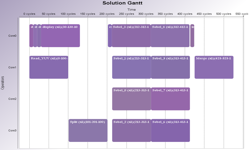
With all actors associated to a 100 µs execution time, we obtain the following schedule where the display actor shares its core with 4 instance of the Sobel actor:
On an 8-cores Intel i7 CPU clocked at 2.40GHz, the execution of this schedule results in the processing of only 1058 fps, which is 2% worse than the performance obtained with the same scenario (100 µs / actor) and 1 pipeline stage (1080 fps).
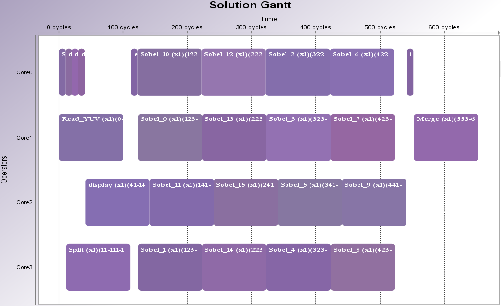
With the 4 cores scenario updated with the measured execution times; we obtain the following schedule where the display actor shares its core with only 3 instances of the Sobel actor:
As a result, on an 8-cores Intel i7 CPU clocked at 2.40GHz, the execution of this schedule reaches 1160 fps, which is 10% better than the previous schedule, but also 5% better than the performance obtained with the same scenario (timed actor) and 1 pipeline stage (1102 fps).