SimSDP: Multinode Design Space Exploration
In this tutorial, you will learn how to use the Simulator for Science Data Processor (SimSDP) to deploy a dataflow application on a heterogeneous multi-node multicore architecture.
The following topics are covered in this tutorial:
- Implementation of a Median Absolute Deviation (MAD)-based Radio Frequency Interference (RFI) filter with PREESM
- Multinode Multicore Partitioning
- Multinode Multicore Code Generation
- Execution on High-Performance Computing (HPC) systems
Prerequisite:
- Install PREESM see getting PREESM
- This tutorial is design for Unix system
Tutorial created the 7.11.2023 by O. Renaud
Introduction
Principle
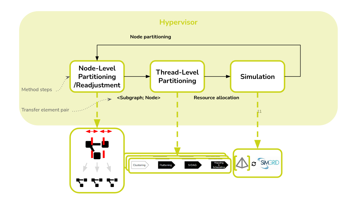
SimSDP is an iterative algorithm integrated into PREESM, designed to achieve load balancing across the available nodes, thereby optimizing performance in terms of final latency [1]. The algorithm steps are as follows:
- Node-Level Partitioning: This step is to divide the graph into subgraphs, each associated with a node.The subgraphs are constructed in such a way as to obtain an balance workload, taking into account the heterogeneity of the nodes.
- Thread-Level Partitioning: Once a subgraph is assigned to a node, we use optimized resource allocation which is a clustering based method called Scaling up of Clusters of Actors on Processing Element (SCAPE).
- Simulation: PREESM simulates both intra-node and inter-node execution, verified by SimGrid, to check if any previously ignored communication affects the final allocation and performance.
- Node-Level Readjustment: Accordingly, the method readjusts the construction of the subgraphs.
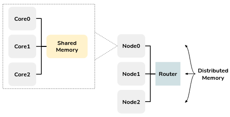
Heterogeneous multi-Node multicore architecture
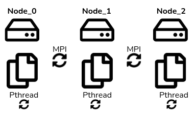
The architectures considered in this tutorial are called heterogeneous multinode multicore architectures. These architectures consist of multiple nodes (or machines), and within each node, there are multiple processing cores. However, what sets this architecture apart is that the nodes and cores are not all identical but rather heterogeneous, meaning they can have different performance characteristics. Notably, communication between cores takes place through shared memory within a node and through distributed memory between nodes as illustrated below.
This architecture is commonly used in high-performance computing (HPC) systems, computing clusters, embedded systems, and other domains where parallelization is essential.
In the rest of this tutorial, we’ll characterize the architecture as follows:
- The number of nodes: This refers to the count of individual machines or computational units in the architecture.
- The internode communication rate: This characterizes the speed at which data can be transmitted between different nodes within the architecture. It is a measure of how fast information can be shared or exchanged between the various nodes.
- The number of core per nodes: This represents the quantity of processing cores (or computing units) present within each individual node.
- The intranode communication rate per node: This indicates the speed at which data can be communicated or shared among the cores within a single node. It measures how quickly cores within the same node can exchange data or work togethe
- The core frequency: Core frequency, often measured in Hertz (Hz), represents the clock speed of each processing core. It determines how quickly the core can execute instructions. Higher core frequencies typically result in faster individual core performance.
- The network topology: Network topologies define the structure of connections and communication pathways between nodes. To narrow the hardware scope of research and cover common usage scenarios, we focus on the five most prominent families of network topologies.
Use-case: Radio-Frequency Interference (RFI) filter
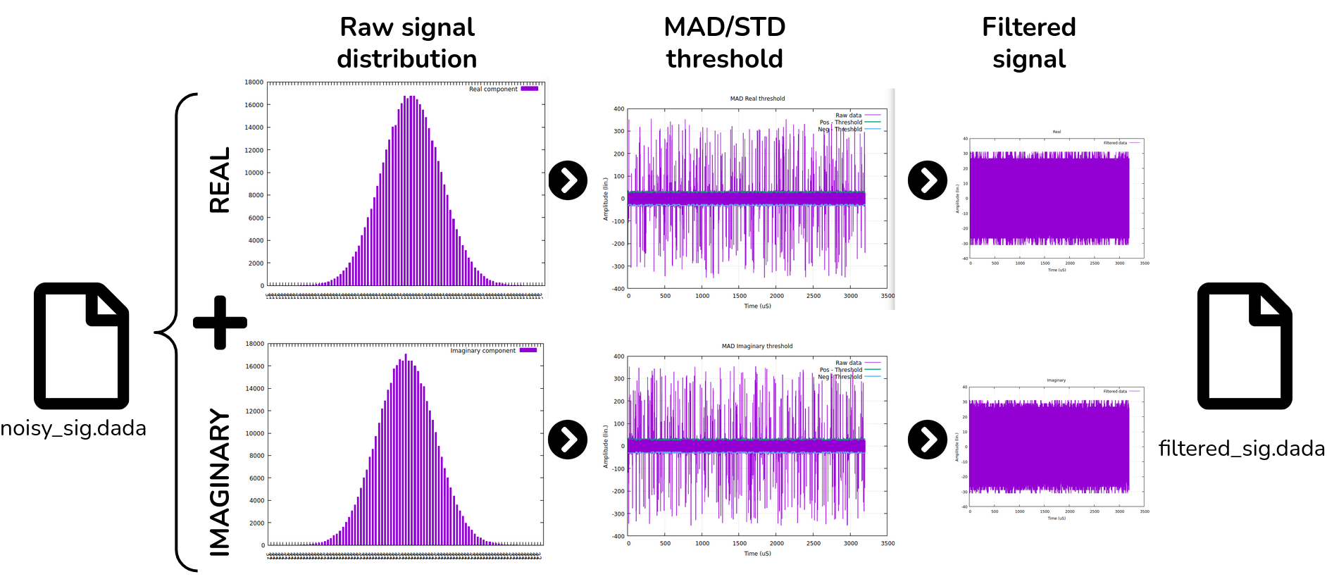
The process involves filtering Radio Frequency Interference (RFI) from an acquisition file obtained by a radio telescope [2]. The file is in the “.dada” format (DADA stand for Distributed Acquisition and Data Analysis) and is comprised of two parts: the header, which contains information about the radio telescope, and the data part. The data part consists of complex numbers. The first step of the process is to separate the real and imaginary components of the data in order to apply filters to both. Two filters are computed simultaneously, and one of them is applied to the data.
- The first filter is the Standard Deviation (STD) filter. See Wiki STD deviation
- The second filter is the Median Average Deviation (MAD) filter. See Wiki MAD deviation.
Both filters aim to find a threshold and remove data points above this threshold. Finally, the filtered real and imaginary parts are combined by taking their conjugates to reconstruct the complex numbers. These reconstructed complex numbers are then used to generate a new “.dada” file.
Project Setup
- Download rfi.pi, and source, and include, and timing here.
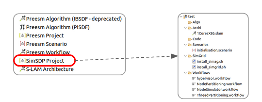
- Launch Preesm and create a simSDP project using “File > New > other… > Preesm > simSDP Project”. Name your project i.e.: “simSDP.RFIfilter” and choose the project location you want.
- Create a CSV file that will be exploit by the method to generate multinode multicore HPC S-LAM files. Name this file “SimSDP_archi.csv” and save it in the Archi folder. Your file should look like this:
Node name;Core ID;Core frequency;Intranode rate;Internode rate Paravance;0;2000.0;472.0;9.42 Paravance;1;2000.0;472.0;9.42 Paravance;2;2000.0;472.0;9.42 Paranoia;4;2000.0;477.6;9.42 Paranoia;5;2000.0;477.6;9.42 Paranoia;6;2000.0;477.6;9.42 Abacus;7;2000.0;1351.68;9.42 Abacus;8;2000.0;1351.68;9.42 Abacus;9;2000.0;1351.68;9.42 -
Configure your network architecture: right click on your project “Preesm > generate custom architecture network”. Choose the network you want. You can let it as default. It generates a XML file stored in the Archi folder (you can update it as you want).
- Add the downloaded files
- In the folder Algo, add rfi.pi
- In the folder Code/source add source
- In the folder Code/include add include
- In the folder Scenario add timing.csv
- file the scenario: open file initialisation.scenario,
- select “overview” browse the algorithm path: rfi.pi, browse the architecture path: temp.slam,
- select “timing” browse the timing file path timing.csv.
You can set the hypervisor to control process iterations:
- Open the workflow “/Workflows/hypervisor.workflow” and select the “hypervisor” task.
- Select “Properties>Task Variables” and customize fields.
| Name | Value | Comment |
|---|---|---|
| Iteration | 5 | It represent a fixed number of iteration. The SimSDP iterative process will stop when this Integer value is achieved. |
| SimGrid | false | True: SimGrid simulate, False : PREESM simulate |
| multinet | false | Enable multiple architecture paths (detail section HPC codesign tool) |
SimGrid provide more accurate simulation in terms of worload,link load, energy and latency and simulate topological networks but only runs on UNIX systems.
Run SimSDP Project
- Right-click on the workflow “/Workflows/hypervisor.workflow” and select “Preesm > Run Workflow”;
- In the scenario selection wizard, select “/Scenarios/initialisation.scenario
During its execution, the workflow will log information into the Console of Preesm. When running a workflow, you should always check this console for warnings and errors (or any other useful information).
Additionnaly, the workflow execution generates intermediary dataflow graphs that can be found in the /Algo/generated/ directory. The C code generated by the workflow is contained in the /Code/generated/ directory. The simulated data are stored in the /Simulation directory.
- Check that you get the tree structure shown below:
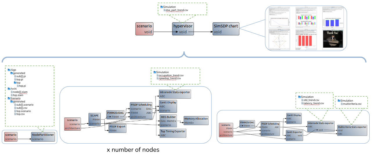
Simulation analysis
At the end of the iterative process (expect about 1 minute per method iteraion), the simulator generate several CSV file.
A python notebook is provided in the SimSDP project.
- To access notebook install the package:
# update package
sudo apt update
sudo apt upgrade
# install python and jupiter notebook
sudo apt-get install python3-pip
pip3 install notebook
- Launch
jupyter notebookand open “SimSDPproject/SimulationAnalysis.ipynb”. Make sure that the CSVs are in the reading path. Load each code to display the trends with your simulated data.
The notebook helps you to analyze:
- The correlation between workload deviation, linkload deviation and latency.
- The duration partitioning of each step of the process to allocate resources.
- The latency trend for each method iteration.
- The memory trend for each method iteration.
- The radar chart of memory vs. final latency vs. cost vs. energy for each simulated architecture deploying your application on the 5 main network topology.
- The occupation trend per node for each method iteration.
- The speedup obtained on each node for each method iteration.
- The workload standard deviation trend between node for each method iteration.
- The workload per node.
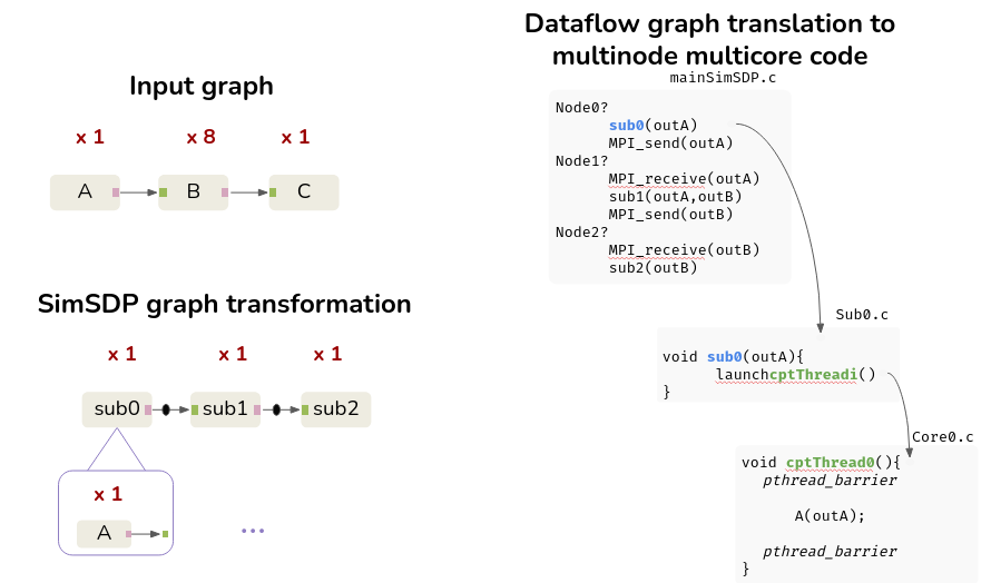
SimSDP code generation
The code generated by SimSDP consists of 3 categories of files. Each machine is in possession of all generated code files. The main file identifies the machine on which it is running via MPI, and calls the functions associated with the node. The sub file contains the thread launch information associated with each node core. The last level is the thread function, which contains the function calls of the placed and scheduled actors. Threads on each machine are synchronized via Pthread, and machines are synchronized via MPI.
Run the generated C Project
In order to run the multicore multinode code in real time, it is necessary to install some libraries, namely “gnuplot” to display the RFI filter curves, “make” to link the files, “pthread” to synchronize the threads, and “mpi” to synchronize the nodes.
- Install dependencies on all the node you will deploy the application:
# install library specific to the application
# install GNU
sudo apt update
sudo apt install -y autotools-dev autoconf libtool make
sudo apt install g++ gfortran
sudo apt install libfftw3-dev pgplot5 libcfitsio-dev
sudo apt-get update
sudo apt-get install gnuplot
#install psrdada
git clone https://git.code.sf.net/p/psrdada/code psrdada
cd psrdada
mkdir build
cd build
cmake ..
make
make install
cd psrdada/build
make install DESTDIR=$HOME

# install make
sudo make install

# install mpi
sudo apt-get install openmpi-bin libopenmpi-dev
(check install: mpicc --version)
(Install pthread see tutorial 01)
- In Code/SimSDPmain.c replace
nodeset["Node0","Node1"]by the name of the nodes
Deploy on the Grid5000 multinode server
Open an account grid5000 account
# ssh connect
ssh orenaud@access.grid5000.fr
ssh rennes
oarsub -I -l nodes=3
# copy file
scp -r ~/path/Code orenaud@access.grid5000.fr:rennes
# compile & run
cd Code/
cmake .
make

# run 2 node each with 1 process
mpirun --mca pml ^ucx --hostfile $OAR_NODEFILE --oversubscribe -n 3 -npernode 1 rfi

# get latency
time mpirun --mca pml ^ucx --hostfile $OAR_NODEFILE --oversubscribe -n 3 -npernode 1 rfi

# get throughput
time mpirun --mca pml ^ucx --hostfile $OAR_NODEFILE --oversubscribe -n 3 -npernode 1 rfi | pv > /dev/null

#get memory static & dynamic
size ./output
valgrind mpirun --hostfile $OAR_NODEFILE --oversubscribe -n 3 -npernode 1 rfi
In the case you want to deploy on specific nodes:
- Check the availability of node or node(production) for rennes (more status here)
- Specify your desire node in the OAR resource manage
oarsub -I -l {"host in ('parasilo-1.rennes.grid5000.fr', 'parasilo-2.rennes.grid5000.fr', 'parasilo-3.rennes.grid5000.fr', 'parasilo-4.rennes.grid5000.fr', 'parasilo-5.rennes.grid5000.fr', 'parasilo-6.rennes.grid5000.fr', 'parasilo-7.rennes.grid5000.fr', 'parasilo-8.rennes.grid5000.fr', 'parasilo-9.rennes.grid5000.fr', 'parasilo-10.rennes.grid5000.fr', 'parasilo-11.rennes.grid5000.fr')"}/host=8
- Visualize specific metrics on the dedicated kwollect dashboard (select your nodes and metric)
In the case you want measure Energy, you should choose to connect Lyon platform such as: gemini, neowise, nova, orion, pyxis, sagittaire, sirius, taurus, wattmetre1, wattmetrev3-1, wattmetrev3-2.
Deploy on random multinode server
Make sure that you have the same mpi version on all your nodes!
# ssh connect
ssh pc-eii114
# copy file
scp -r ~/path/Code orenaud@pc-eii114:path/Code
# compile & run
cd Code/
cmake .
make
mpirun -np 3 -host po-eii26,pc-eii114,pc-eii27 ./output
# if you have just 1 node at your disposal (and you just want to test the output)
mpirun -np 3 ./output
Running the application in parallel will display a succession of 6 graphics.
the sky images are collected and stored in a .dada file. By separating the imaginary part of these images, we observe a heavy-tailed Gaussian distribution (ref.: the first 2 graphs). This type of distribution is typical of RFI due to the nature of the sources that generate the interference and the propagation characteristics of the interfering signals. The use of MAD or STD filters is justified by their robustness in the face of outliers, particularly in the extreme values of heavy-tailed distributions that affect conventional estimators. These 2 filters are then applied and displayed on the next 2 graphs. The best-performing filter is then selected for final filtering (ref. the last 2 garphics). The filtered signal is then reconstituted by combining the two parts to form a new .dada file.
HPC codesign tool
Because performance depend on both an efficient workload partitioning and an appropriate target architecture SimSDP has been extended to automatically retrieve a multinode architecture providing the best final latency for a given application [3] . The extension add two primary steps to the initial method in order to define a architecture search strategy namely, Scope Initialisation and Scope Readjustment. The extension also an in depth analysis of the architectures parameters impact by fine-tuning the Simulation step.
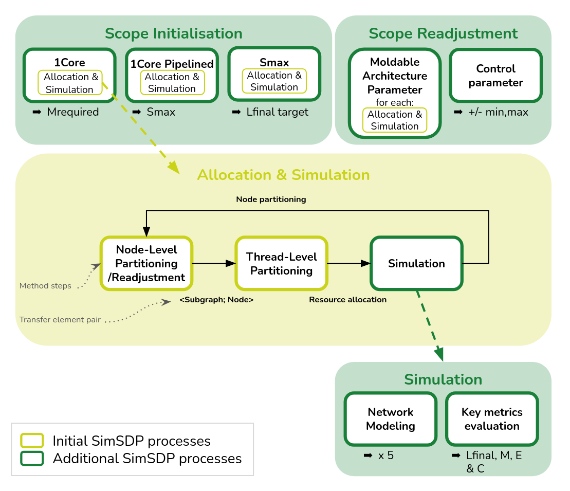
- Scope Initialisation: This step involves the deployment of a specified application on a single-core architecture to compute the minimal memory required and the estimated maximal final latency speedup for a given application composing the exploration boundaries.
- Scope Readjustment: The subsequent steps involve the iterative deployment of the application on a range of multinode architectures, where architecture parameters are initially set and then refined.
- Simulation: For each architecture, the tool allocates resources thanks to our previous work and conducts simulations for four key metrics across five main network topologie.
Project Setup
In order to set up the codesign process.
- Keep your former SimSDP project.
- Add a SimSDP_moldable.csv in the Archi folder which should look something like this:
| Parameters | min | max | step |
|---|---|---|---|
| number of nodes | 1 | 6 | 1 |
| number of cores | 1 | 6 | 1 |
| core frequency | 1 | 1 | 1 |
| network topology | 1 | 4 | 1 |
| node memory | 1000000000 | 1000000000 | 1000000000 |
- Change the hypervisor parameter: select the “hypervisor” task, select “Properties>Task Variables”
| Name | Value | Comment |
|---|---|---|
| Iteration | 1 | It represent a fixed number of iteration. The SimSDP iterative process will stop when this Integer value is achieved. |
| SimGrid | true | True: SimGrid simulate, False : PREESM simulate |
| multinet | true | enable multiple architecture paths |
- Run the hypervisor workflow with the Initialisation scenario.
Wait a moment, the tool will scan the architecture until it finds the optimal one and display the pareto analysis.