CPU-GPU Design Space Exploration
In this tutorial, you will learn how to use the Scaling-up of Cluster of Actors on Processing Element (SCAPE) method to deploy a dataflow application on a heterogeneous CPU-GPU architecture.
The following topics are covered in this tutorial:
- Implementation of a Distributed FX (DiFX) correlator with PREESM
- Heterogeneous CPU-GPU Partitioning
- Heterogeneous CPU-GPU Code Generation
- Execution on laptop or High-Performance Computing (HPC) systems
Prerequisite:
- Install PREESM see getting PREESM
- This tutorial is design for Unix system
Tutorial created the 8.5.2024 by O. Renaud & E. Michel
Introduction
Principle
SCAPE is a clustering method integrated into PREESM, designed to partitioning GPU-on-GPU compatible computations and CPU-on-CPU compatible computations, evaluating offloading gains and adjusting granularity [1]. The method happens upstream of the standard resource allocation process. It takes as input the GPU-oriented System-Level Architecture Model (GSLA) Model of Architecture (MoA) and the dataflow MoC and partially replicates the standard steps avoiding the need for a complete flattening such as:
- Extraction:
- GPU-friendly pattern identification: This task identifies data parallel patterns such as URC and SRV as suitable dataflow models for GPUs as introduced in Section II-E.
- Subgraph generation: The identified actors are then isolated into a subgraph where rates are adjusted to contain all data parallelism.
- Scheduling: The chosen scheduling strategy for the cluster is the APGAN method.
- Timing: This step estimates the execution time of the subgraph running on a GPU, considering memory transfers between GPUs during execution.
- Mapping: This task estimates parallelism gain and transfer loss based on GSLA information. If GPU offloading is beneficial, the process proceeds; otherwise, the original SCAPE generates a cluster of actors mapped on CPU.
- Translation: The subgraph is translated into a CUDA file and sent to the rest of the resource allocation process after transformation, simplification, and optimization.
GSLA MoA
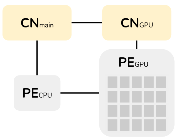
The System-Level Architecture Model (S-LAM) provides a structured framework for system architectures, including subsets like the Linear System-Level Architecture Model (LSLA) and the GPU-oriented System-Level Architecture Model (GSLA). GSLA allows internal parallelism modeling in Processing Elements (PEs), while LSLA requires modeling all PEs for reliability, leading to differences in cost definition. LSLA for GPUs requires modeling each kernel element as a processing element, making mapping and scheduling complex. We choose GSLA for this method because it handles complexities better while preserving data parallelism.
Below is a GSLA representation compose of one CPU core , one GPU kernel, one main communication node and one GPU communication node:
Use-case: DiFX correlator
The principle of the core of DiFX [2][3] is the following :
- Data Alignment: Given the vast distances separating telescopes, signals they record may encounter delays due to varied travel paths. The correlator aligns these signals in time to ensure synchronicity with the observation moment.
- Correlation: Once aligned, the correlator compares signals from each telescope, performing mathematical correlation by multiplying and summing received signals over a specific time interval.
- Image Formation: Correlated data provide insights into the brightness and structure of observed astronomical objects.
Below is a simplified dataflow representation:
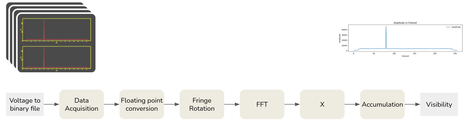
Data Acquisition: Telescope data is retrieved from disk in binary format, devoid of headers. Each binary file (xx.bin) is packed into a 2D array, with one file per antenna. Subsequently, delays between telescopes are computed based on a polynomial from the configuration file (xx.conf).
Floating Point Conversion: Raw integer-encoded data is converted to floating-point numbers. This stage also creates complex numbers with zero imaginary values and divides data into independent channels, stored in a 3D array per polarization per antenna. An “offset” correction is applied to account for geometric signal reception time effects.
Fringe Rotation: Each sample undergoes ‘fringe rotation’ to adjust for telescopes’ relative speeds (Doppler shift). This involves applying a time-varying phase shift to each sample.
FFT of Samples: “N” time samples are transformed into frequency-domain data, making it easier to extract information later.
Cross-correlation (X): Individual frequency channels of each telescope are multiplied and accumulated to form “visibilities” for each FFT block. This process generates unique baselines combinations and integrates sub-integration data over milliseconds, averaged for approximately one second to form the final visibility integration.
Accumulation: Cross-correlation values for each FFT block are added to previous iterations in the “visibilities” table, resulting in final visibility products. Phase and amplitude data for each frequency channel and baseline are stored in a vis.out file.
(more detail on running different DiFX implementation can be found on the readme of the DiFX dataflow model, notably FxCorr and Gcorr)
Project Setup
- Download DiFX project from Preesm-apps
- Launch Preesm and open the project: Click on “File / Import …”, then “General / Existing Projects into Workspace” then locate and import the “org.ietr.preesm.difx” project
-
Create an GPU-accelerated architecture. Based on a classic CPU architecture: “right click on architecture > generate a custom x86 architecture > select 1 core”. Select the GPU vertice from the palette and drop it on your design. Select a parallelComNode and drop it to your design. Connect each element with undirectedDataLink. Take the figure below as an example.
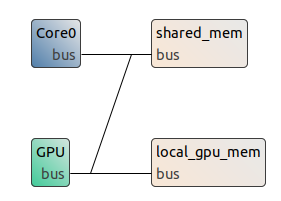
- Custom you GPU node: select the node and ajust the parameter to fit your target.
| Property | Value | Comment |
|---|---|---|
| dedicatedMemSpeed | 20000 | Speed of the dedicated memory (in MB/s), typically higher than unified memory. |
| definition | defaultGPU | |
| hardwareId | 1 | Unique identifier for the GPU hardware. |
| id | GPU | Identifier name for the GPU in the system configuration. |
| memoryToUse | dedicated | Specify memory allocation type: “dedicated” for GPU-exclusive memory or “unified” for shared CPU-GPU memory. |
| memSize | 4000 | Size of the GPU’s memory (in MB), determining the amount of data it can handle. |
| unifiedMemSpeed | 500 | Speed of the unified memory (in MB/s), typically slower but shared between CPU and GPU. |
- Generate your scenario: right click on your project “Preesm >generate all scenarios.
- Custom the Codegen.workflow to generate the appropriated CPU-GPU code:
- Open the Codegen.workflow
- Add a new Task vertex to your workflow and name it SCAPE. To do so, simply click on “Task” in the Palette on the right of the editor then click anywhere in the editor.
- Select the new task vertex. In the “Basic” tab of its “Properties”, set the value of the field “plugin identifier” to “scape.task.identifier”.
- In the “Task Variables” tab of its “Properties”, fill the varaible like this:
Parameter Value Comment Level number 0 Corresponds to the hierarchical level to coarsely cluster, works with all SCAPE mode 0, 1 and 2. SCAPE mode 0 0: match data parallelism to the target on specified level, 1: match data and pipeline parallelism to the target on specified level, 2: match data and pipeline parallelism to the target on all admissible level. Stack size 1000000 Cluster-internal buffers are allocated statically up to this value, then dynamically.
(more detail, see Workflow Tasks Reference )
- connect the new task to the “scenario” task vertex and to the “PiMM2SrDAG” task vertex as shown in the figure below.
[here insert a figure] - Right-click on the workflow “/Workflows/Codegen.workflow” and select “Preesm > Run Workflow”;
The workflow execution generates intermediary dataflow graphs that can be found in the “/Algo/generated/” directory. The C code generated by the workflow is contained in the “/Code/generated/” directory.
Execution of the DiFX correlator dataflow model
- Download the IPP (Intel Integrated Performance Primitives for Linux ,2021.11.0,19 MB,Online,Mar. 27, 2024):
chmod +x l_ipp_oneapi_p_2021.11.0.532.sh
./l_ipp_oneapi_p_2021.11.0.532.sh
Execution on laptop equiped with GPU
- Check if your laptop is equiped with Nvidia GPU :
lspci | grep -i nvidiaPrompt:
3D controller: NVIDIA Corporation GA107M [GeForce RTX 2050] (rev a1)
- Install NVIDIA CUDA Drivers & CUDA Toolkit for your system, see NVIDIA’s tutorial
- Check CUDA compiler & CUDA install with
nvcc -VPrompt:
→ nvcc: NVIDIA (R) Cuda compiler driver
→ Copyright (c) 2005-2024 NVIDIA Corporation
→ Built on Thu_Mar_28_02:18:24_PDT_2024
→ Cuda compilation tools, release 12.4, V12.4.131
→ Build cuda_12.4.r12.4/compiler.34097967_0
A MakeFile is stored on the /Code folder
- correct the IPP path to your IPP path
- Compile and run
cmake .
make
./difx
Execution on Grid5000
- Open an account grid5000 account.
The example here are for rennes.
- Choose the node you need based on its characteristics (number of GPUs, memory …) presented in Rennes:Hardware - grid5000.
Check the availability of yourchosennode on Rennes:node or Rennes:node(production)
(more status here)# ssh connect ssh orenaud@access.grid5000.fr ssh rennes #connect 1 abacus node (they host NVIDIA GPU) oarsub -q production -p abacus1 -I #copy the folder scp -r ~/path/Code orenaud@access.grid5000.fr:rennes
A MakeFile is stored on the /Code folder
- correct the IPP path to your IPP path (download IPP on the machine)
- Compile and run
cmake .
make
./difx
DiFX execution generates a file containing visibility information vis.out
Display results
You can visualize your data with the notebook available here.
Import your vis.out file and run the code.
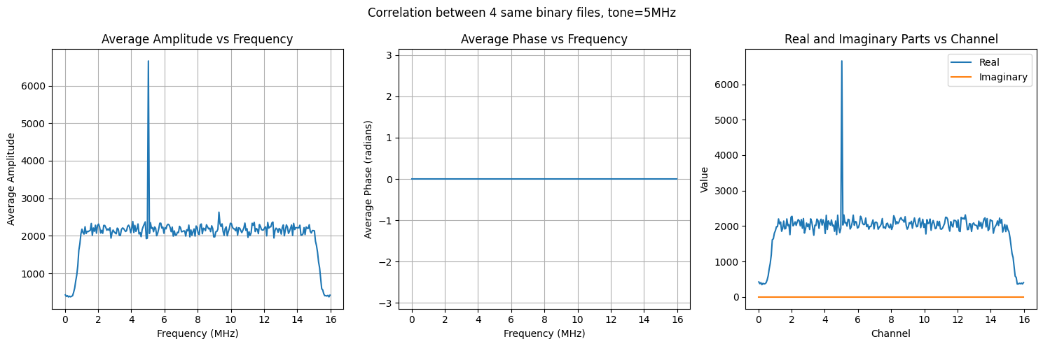
Display of the 4 average caracheristics by baselines (detailed in the notebook).
To run the original version of FxCorr and Gcorr follow the readme of the DiFX dataflow model stored on preesm-apps.
References


Acknowledgement
This project has received funding from the European Union’s Horizon 2020 research and innovation program under the Marie Skłodowska-Curie grant agreement No 873120.